Internet Educational Series #10: Routing

1. Shortest Path Algorithms (SPAs)

In graph theory, the shortest path problem is the problem of finding a path between two vertices (or nodes) in a graph such that the sum of the weights of its constituent edges is minimized. Common algorithms for solving the shortest path problem include the Bellman-Ford algorithm and Dijkstra’s algorithm.

Bellman-Ford

This algorithm aims to find the shortest path to go from a source (s) to any destination in a certain topology.

Topologies are composed of vertex (nodes) and edges (links).

There are 2 different versions of topologies. Centralized ones, where the source node knows the whole topology, and distributed ones. In the latest version, a node wants to compute the shortest path to other nodes, but without knowing the whole topology, the source node will only have the estimated distances provided by its neighbors.

To explain it in plain words, the neighbor nodes exchange their vector of distances between them:

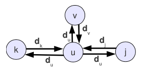
When a node u receives the vector of distances dk from its neighbor k. it can use the distances on this vector to relax the edge to this neighbor (u,k).

Let’s see an example of a topology that uses the distributed version of BF to show the distribution of the route to the node a. You’ll see the update messages and the route to the node a that each node learns when the distance vectors are exchanged between them.

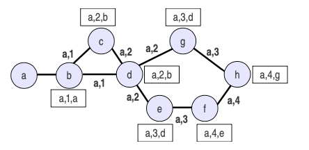
Notice the decentralized computation: d sends only the best path to a.

Process:

• b relaxes (a,b) and sends the update to its neighbors.
• d receives the previous update from b and then relaxes (d,b) and sends the update to its neighbors.
• g receives the previous update from d and then relaxes (g, d) and sends the update to its neighbors.
• h receives the previous update from g and relaxes (h,g).

See how the algorithm converges to the optimal solution (shortest path) because this decentralized process? It runs BF in an end-less loop in which each node relaxes its edges.

Once all nodes have sent and received update messages it turns out to be like an iteration of the centralized algorithm.

Dijkstra

This is another algorithm to find the shortest path to go from a source (s) to any destination in a certain topology.

The difference between this one and BF, is that Dijkstra only works in topologies that are free of edges with negative weights.

Let’s see an example of how Dijkstra algorithm works in the following topology:

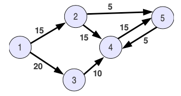
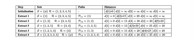
When we initialize the algorithm, there are no sources, and the only “reachable” destination is node1.

• In the first iteration, we find the distance between 1–2 and 1–3. The path cell tells us that the only “shortest path” available now is how to reach node1 (only 1 hop without weight).
• Extract 2 shows that we do now have 2 sources to reach the nodes 3, 4 and 5, and that the shortest path uses nodes 1 and 2 to reach node 5.
• Extract 5 has node 5 as a source now. However instead of going for node4, it detects that now the shortest path (the one with less weight) is node3, so it adds the distance to reach node3 from node1, instead of adding the distance to the direct neighbor from the previous extract.
• Extract 3 is the last one that is looking for a route to reach the only missing node (4). It calculates that the shortest path to reach node 4 is through nodes 2 and 5, instead of node 3.
• Finally we do have all the distances between the nodes from the topology, and the shortest paths to reach each one of them.

Great, now that you have had a quick glimpse on SPAs, let’s get into the real matter of this article. Routing Information Protocol (RIP).

2. RIP

The Routing Information Protocol is a dynamic routing protocol that is used in small/medium IP networks. It is based on a distance-vector exchange, and a distributed version of BF.

RIP has been evolving during the years, and new versions have been surging, like RIPv2, RIPng (RIP next generation), which has been adapted for IPv6, and lately another protocol called OSPF has been gaining popularity. However, to understand all of the above, we need to know how the basic form of routing works.

RIP, like any other routing protocol, defines a routing database, a protocol for exchanging information about routes and an algorithm for updating routing information.

We will describe these three parts below:

2.1 Routing Database

Each RIP entity (normally routers) keep track in its routing database of all networks (and possibly individual hosts) in the RIP routing domain.

Each entry in the routing database includes the next intermediary router (called next hop) to which datagrams have to be delivered so that they can reach the final destination. In addition, the routing database includes a metric for measuring the total distance to the final destination.

The fields specified in the routing database are:

• Address. Destination network or host. (@IP/MASK)
• Metric. The metric or cost from that node to the destination.*
• Router. Next-hop to reach the destination network or host.
• Interface. The network interface that must be used to reach the next router.
• Timers. Used to manage dynamics of the routing information.

*The metric is basically the number of hops to the destination. A datagram makes a hop when it goes through a router. For example, if a RIP entity is directly connected to its destination, the distance is 1 hop, but if the source and destination are connected through another intermediary router, then the distance is 2 hops.

The valid metrics range is between 1 and 16 hops, however the maximum number of hops allowed for any destination is 15, and the distance 16 is reserved for “infinity”, in other words, destination unreachable.

2.2 Updating Algorithm

This is the part where RIP gets fun (at least for coders/technical people ;) ).

Distance vectors algorithms get their name from the fact that it is possible to compute optimal routes by periodically exchanging the vector of distances to the different destinations that each node in the network has.

The Routing Database of each RIP node is initialized with a description of the RIP entities that are directly connected (next-hop=1), and then it updates with a distributed version of BF.

However, what happens if the network we are in changes, a RIP entity disconnects, disappears, or another entity gets inside the network and then there is a better optimal path?

Let’s first explain how the algorithm behaves in a static topology, and then we’ll dive deeper into dynamic topologies and the problems that we may find.

Static Topology

Let’s first define some variables. w(i,k) is the weight or cost of the edge that connects nodes i and k. So w(i, k) = 1 if i and k are directly connected and w(i, k) = 16 (infinity) if they are not. Moreover, m(P(i,j)) as the best current metric for the path or route between i and j.

The Bellman-ford equation and it says that “the best route is through the neighbor that has the minimum distance to the destination”.

So, when a RIP entity i receives the distance vector dk with the estimates of neighbor k, it adds w(i, k) to each of the estimations received. Then, for each destination n, the node i compares the metric provided by the neighbor with its current routing entry metric for this destination R(n).metric. The node picks the new route if the metric provided by the neighbor is smaller. With this algorithm, after receiving estimates from all the nodes in the network, i will have the smallest distance to all the destinations.

Dynamic Topology

Decrease the metric

The method so far only has a way to lower the metric, as the existing metric is kept until a smaller one shows up.

However, it is possible that the initial estimate might be too low. In this case, we need a method for “increasing the metric”.

For this purpose, it is enough to always consider the information received by the next hop of a route. For example, suppose the current route to a destination has metric D and uses router R. If a new set of information arrived from some source other than R, only update the route if the new metric is better than D. But if a new set of information arrives from R itself, always update D to the new value.

Updates

It is safe to run the algorithm asynchronously, that is, each RIP entity can send updates with its distance vector according to its own clock. The algorithm will converge to the correct distances in finite time in the absence of topology changes.

Originally each RIP router transmitted full updates every 30 seconds. In the early deployments, routing tables were small enough that the traffic was not significant. As networks grew in size, however, it became evident there could be a massive traffic burst every 30 seconds, even if the routers had been initialized at random times.

Modern RIP implementations introduce deliberate variation into the update timer intervals of each router.

Example

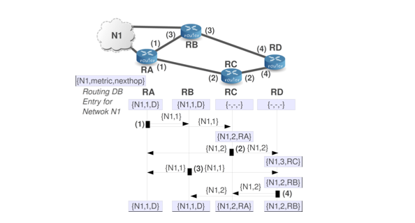
As you can see, N1 is connected to RA and RB. We are going to illustrate how the information about Network 1 (N1) can be distributed by RIP. As the order of the RIP updates is randomly distributed (unpredictable), the description that follows is just a possible realization of the RIP update process.

Let’s go step by step:

(1) As initial condition we assume that the only routers that have information about N1 are the two directly connected routers (RA and RB). Then, RA is the first router to send information about N1 in a RIP message (in this case, but RB could also be the first one). We will note this information as {N1,1}, which means that the RIP message sent by RA includes an entry for N1 showing that this router can reach this network with one hop. RA sends this RIP message to its one-hop neighbors: RB and RC. Upon receiving this information, RC updates its routing database because the information received by RA informs about a new reachable network. RB does nothing because it already knows N1 with a better (shorter) path.

(2) RC decides that it has to send a RIP message and it includes the new information it knows about N1. This information is that it can reach N1 with two hops {N1,2}. RC sends this information to its one-hop neighbors: RA and RD. In the case of RD, this is the first time it hears about N1, so it updates its routing database with the new information. Obviously, RA does nothing.

(3) This time RB sends its RIP message including the entry {N1,1} to its one-hop neighbors: RA and RD. RA does nothing, but RD updates its routing database because the new information from RB provides a shortest path to the destination than the previous one that RD possessed.

(4) This time RD sends its RIP message but nobody does nothing because the information provided by the router is worse than the information present at the routing databases of the rest of the routers (this is logical because RD is the farthest router).

BROKEN LINK

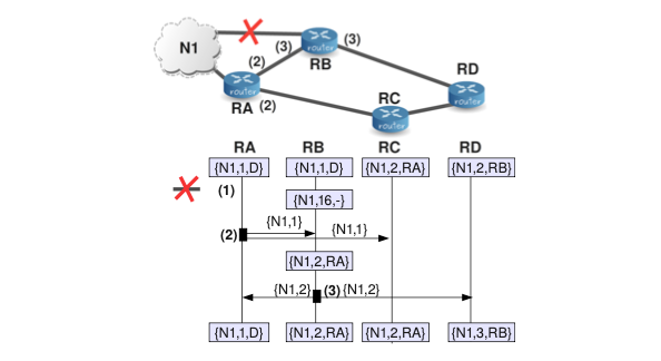
Now, we are going to assume that one of the links is broken. In particular, the link that connected RB to N1.

In this case, we are going to observe that some nodes have too low estimations for N1 and we will see how nodes use the method for increasing the metric. The description that follows is a possible realization of the RIP update process:

(1) As an initial condition, we assume that all the routers have converged to the topology depicted in the first example. Thus, they have entries for N1. Then, RB detects that its link to N1 is broken. At this moment, RB updates the entry for N1 in its database setting the metric for this network to infinity (16).

(2) RA sends a RIP message to its one-hop neighbors: RB and RC. Upon receiving this information, RB updates its routing database because the information received by RA informs about a new path to reach again the network N1. RC does nothing because it already knows N1 with the same metric.

(3) At this time RB sends a RIP message to its one-hop neighbors: RA and RD. RA does nothing, but RD updates its routing database because although the information received contains a worse metric, it comes from the next hop router. Recall that according to the “increasing metric method”, we always have to update our routing entries when the information comes from the next hop. Notice also that this can be interpreted as an indication that our estimate for N1 is currently too low. Indeed, with the new network topology, RD cannot reach N1 with just two hops.

2.3 Improvements

In practice, routers and lines often fail and come back up. To properly handle dynamisms the algorithm presented so far is not yet suitable and some enhancements are required.

1. TIMERS

Notice that if a certain router X is included in the best route to a certain destination of some other router Y , and the router X is no longer available (for example because it crashed or because some network connection to it is broken), the algorithm explained so far might never reflect the change to router Y . The algorithm as shown so far depends upon routers notifying its neighbors if their metrics change. In order to handle problems of this kind, distance vector protocols must make some provision for timing out routes. For this purpose, there are two timers associated with each route: a “timeout” and a “garbage-collection” time.

• The timeout is used to limit the amount of time a route can stay in a routing database without being updated. Recall that RIP entities have to send update messages approximately every 30 seconds. The timeout is initialized to 180 seconds whenever a new route is established and is reset to the initial value whenever an update is heard for that route. If an update for a route is not heard within that 180 seconds (six update periods), the hop count for the route is changed to 16, marking the route as unreachable.
• The other timer, the garbage collection timer, is used to make help neighbors making them know that the route is no longer valid. An unreachable route will be advertised with the infinite metric (16) until the garbage-collection timer expires (120 seconds by default). After this, the route is removed from the route database.

2. COUNT TO INFINITY

To illustrate this problem, we continue our example but this time we “break“ the link between RA and N1. As a result is broken, N1 is now unreachable for our four RIP routers.

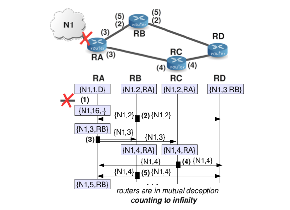
(1) As shown in the image above, at a certain moment the last link to N1 is broken. At this moment, RA, who is the only one-hop RIP neighbor of N1 detects this situation and sets the metric for this network to infinity in its routing database.

(2) At a certain moment, RB sends a RIP message with its current information about N1. That is to say, RB sends {N1,2} since it has not received any new information about N1. This out-of-date information arrives to RA since it is a one-hop neighbor of RB, and it causes the update of the RA’s entry for N1.

(3) RA sends its RIP update message including {N1,3}. This causes an update in the entries for N1 in RB and RC.

(4) RC sends its RIP update message including {N1,4}, which does not cause any update in the neighbors.

(5) RB sends its RIP update message including {N1,4}, which causes that RA increases the metric for this network up to 5. At this moment, RA and RB are in mutual deception because each mutual RIP update message causes an increase of the metric for the N1 network in the other neighbor.

Notice that the behavior of algorithm is correct in the sense that the network is now at a distance of infinity and in fact, with the successive updates, the metric for the route is slowly increasing to infinity. However, we have a problem because the “counting to infinity” will never end and thus the routing databases will never converge. Thus, at this point it might become clear why we have to limit the maximum number of hops of a RIP domain and why “infinity” should be chosen as small as possible. Notice however, that infinity must be large enough so that no real route is that big. Therefore, the choice of infinity is a trade-off between network size and speed of convergence in case counting to infinity happens. The designers of RIP believed that the protocol was unlikely to be practical for networks with a diameter larger than 15, and thus they decided to set infinity to 16.

3. SPLIT HORIZON

The counting to infinity problem that we saw in our previous example is caused by the fact that RA and RC are engaged in a pattern of mutual deception. Each claims to be able to get to N1 via the other. This can be prevented in many cases by being a bit more careful about which information is sent to which neighbors.

In general, the idea of providing a ”split view“ of your available information receives the name of ”split horizon”. In the context networking, split horizon is used to solve several problems and also to provide certain functionalities. In the context of RIP, in its simplest version, the split horizon rule is just to omit routes learned from one neighbor in updates sent to that neighbor. The reason for this, is that it is never useful to send information about a certain route to the neighbor that you are using as next hop for the route in question. Let illustrate this technique with an example:

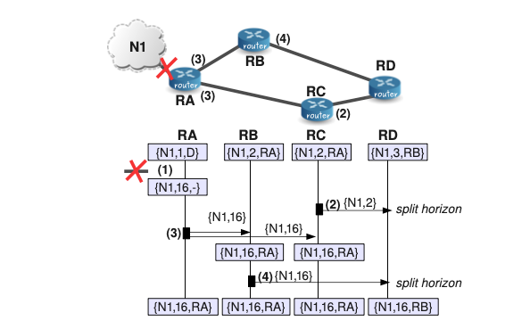
(1) At a certain moment the last link to N1 is broken. At this moment, RA, who is the only one-hop RIP neighbor of N1 detects this situation and sets the metric for this network to infinity in its routing database.

(2) At a certain moment, RC sends a RIP message with its current information about N1 but in this case RC applies the split horizon rule and thus, it sends information about N1 only RD and not to RA because RA is the next hop for N1 in the RB’s routing database. This avoids contaminating the routing entry for N1 of RA with out-of-date information coming from RC.

(3) RA sends its update to its neighbors RB and RC. After receiving the update, RB and RC update their routing databases because both had RA as next hop router (they apply the “increasing the metric rule”).

(4) Using the simple split horizon rule, RB sends its update to RD. The final result is that RD updates its routing entry for N1 and that all the routers in the RIP domain know now that N1 is unreachable.

The simplest version of split horizon prevents the majority of the situations of mutual deception. However, in the eventual situation in which a router, say RC, thinks that it can get a network, say N1, via another router, say RD, and RD thinks that it can get N1 via RC, in this case, we have a loop. For solving this situation, the standard of RIP proposes a modification in the behavior of split horizon called “split horizon with poisoned reverse”. With poisoned reverse, there is also an “split view” of routing information available, but the idea is not omitting routes learned from one neighbor in updates sent to that neighbor but include them with their metrics set to infinity.

3.1 Split Horizon with poisoned reverse

Let’s see a particular way in which we might arrive to a situation of mutual deception although we have activated split horizon. Then, we show how activating split horizon with poison reverse might help. For this example, we are considering that packets that convey the RIP update data may suffer delays.

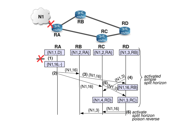
These delays are typically due to the process of transmitting the data through the network and also to the time spent by the packets at different queues at the sender and the receiver. These delays also cause that RIP update messages sent to a neighbor are not immediately received and processed by that neighbor.

Let’s describe the situation:

(1) As mentioned, we consider at a first moment that only the simple split horizon is activated. Then, at a certain moment, the last link to N1 is broken. At this moment, RA, who is the only one-hop RIP neighbor of N1 detects this situation and sets the metric for this network to infinity in its routing database.

(2) RA sends RIP update messages containing the entry {N1,16} to neighbors RB and RC. As it is shown in Figure 2.5, these update messages arrive to the neighbors at different instants of time.

(3) RB after receiving and updating its entry for N1 to infinity, RB sends a message to its neighbor RD. Notice that RB does not send any update message to RA since slit horizon is activated.

(4) RD sends an update to RC including {N1,3}, just a little bit before receiving the update for N1 from RB. As split horizon is activated, RD does not send information about N1 to RB. The update from RD is received by RC after the update from RA, and thus, the entry in the RC’s database for N1 is {N1,4,RD}.

(5) RC sends and update about N1 to RD just before receiving the update from RA telling that N1 is unreachable. As a result, RC will end with an entry for N1 that is {N1,3,RC}. At this point, RC and RD are in mutual deception. Furthermore, they will not send to each other any update message because of the split horizon rule. Therefore, to clean the route N1 from the routing tables, we will have to wait to the timeout.

(6) In the final step, we see that if we activate split horizon with poison reverse, RD might send an update message to RC and remove the loop with RC before the timeout for the route expires.

Certainly it is rather improbable that with simple split horizon activated two routers end with routes pointing at each other, but it can happen.

In general, split horizon with poisoned reverse is safer than simple split horizon because advertising reverse routes with a metric of 16 will break any loop of mutual deception between two routers immediately. If the reverse routes are simply not advertised, the erroneous routes will have to be eliminated by waiting for a timeout.

4. TRIGGERED UPDATES

Split horizon with poisoned reverse will prevent routing loops that involve two routers. However, it is still possible to end up with patterns in which three routers are engaged in mutual deception.

Triggered updates are used to speed up convergence by avoiding that out-of-date updates produce patterns of three or more routers in mutual deception. To implement triggered updates, we simply add a rule that whenever a router changes the metric for a route, it is required to send update messages to its neighbors almost immediately, even if it is not yet time for a regular update message.

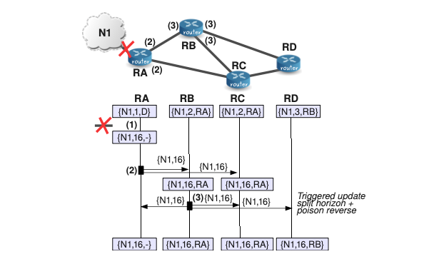
(1) After the link to N1 is broken, RA sets the metric for this network to infinity in its routing database.

(2) RA sends an update about N1 to its neighbors RB and RC. Since this update message causes a change of metric for the entries of network N1 in RB and RC, these routers must “immediately” send a triggered update for this network.

(3) In particular, we can observe that after RB sends its triggered update and this message is processed, all the routers in the RIP routing domain have already converged to the correct metric (16) for N1.

Notice that if the system does not send any regular update while the triggered updates are being sent, it would work perfectly.

Unfortunately, things are not so nice. While the triggered updates are being sent, regular updates may be happening at the same time. Routers that haven’t received the triggered update yet will still be sending out information based on the route that no longer exists. It is possible that after the triggered update has gone through a router, it might receive a normal update from one of these routers that hasn’t yet gotten the word. This could reestablish an out-of-date version of the faulty route. If triggered updates happen quickly enough, this is very unlikely. However, counting to infinity is still possible.

The final aspect about triggered updates to be taken into account is related to performance. Triggered updates can cause excessive load on networks with limited capacity or networks with many routers on them. This is due to the fact that triggered updates cause a lot of network traffic in a short period of time. Therefore, the protocol requires that implementors include some mechanisms to avoid these performance problems. To this respect, the standard proposes two mechanisms:

• The first mechanism is to limit the frequency of triggered updates. After a triggered update is sent, a timer should be set for a random interval between 1 and 5 seconds. If other changes that would trigger updates occur before the timer expires, a single update is triggered when the timer expires. The timer is then reset to another random value between 1 and 5 seconds. Furthermore, a triggered update should be suppressed if a regular update is due by the time the triggered update would be sent.
• The second mechanism says that triggered updates do not need to include the entire routing table. In principle, only those routes which have changed need to be included. Therefore, messages generated as part of a triggered update must include at least those routes that have their route change flag set. Split Horizon processing is done when generating triggered updates as well as normal updates. The only difference between a triggered update and other update messages is the possible omission of routes that have not changed. The remaining mechanisms must be applied to all updates.

5. HOLD DOWN TIMER

As a final enhancement, we will explain the Hold Down Timer mechanism:

Each router starts the hold-down timer when it first receives information about a network that is no longer reachable (RIP distance=16). Until the hold-down timer expires, the router will discard any subsequent update messages that indicate the route is again reachable. A typical hold-down timer ranges from 60 to 120 seconds. The main advantage of the hold-down timer is that a router will not be confused by receiving spurious information about a route being accessible, when it was just recently told that the route was no longer valid. This provides a period of time for out-of-date information to be flushed from the system. However, this has a disadvantage because the hold-down timer forces a delay in a router responding to a route once it is fixed. For example, let us suppose that a network “hiccup” causes a route to go down for five seconds. After the network is up again, the hold-down timer must expire before the router will try to use that network again. This makes using hold-down relatively slow to respond and may lead to delays in accessing networks that fail intermittently.

2.4 RIP History

Great, now we’ve seen the different mechanisms that the RIP uses. Let’s now explain how does the protocol itself, and the main improvements made in each version.

RIP messages are sent using the User Datagram Protocol (UDP) with UDP port number 520 for RIP-1 and RIP-2, and 521 for RIPng. Notice that even though RIP is considered part of layer three, in terms of message exchange, RIP behaves like an application (using UDP/IP). The format of RIP messages is version-dependent. On the other hand, RIP messages can be either sent to a specific RIP neighbor (unicast), or they can be sent to multiple neighbors (broadcast or multicast). For the three versions of RIP, we have only two basic types of messages:

• RIP Requests. Requests are messages sent by a RIP entity to another RIP entity asking it to send back all or part of its routing table.
• RIP Responses. Responses are messages sent by a RIP entity containing all or part of its routing table. Despite the name “response”, as we have already seen, these messages are sent most of the time without any preceding request.

RIP-1

RIP-1, the original specification of RIP uses classful network addresses because the message format of RIP-1 does not consider sending masks. As a result, this protocol lacks support for subnetting or supernetting. Another limitation of RIP-1 is that there is not support for router authentication, making RIP vulnerable to various attacks.

RIP messages are sent using the UDP/IP network. Regarding the IP layer, the RIP-1 entity can select a unicast transmission by setting the destination IP of the neighbor or a broadcast transmission by setting the universal broadcast IP address 255.255.255.255. Regarding the UDP layer, RIP-1 uses the UDP reserved port number 520. The UDP port numbers in RIP-1 are used as follows:

• RIP Request messages are sent to UDP destination port 520. They may have a source port of 520 or may use an ephemeral port number.
• RIP Response messages sent in reply to an RIP Request are sent with a source port of 520, and a destination port equal to whatever source port the RIP Request used.
• Unsolicited RIP Response messages (sent on a routine basis and not in response to a request) are sent with both the source and destination ports set to 520.

RIP-2

RIP-2 represents a very modest change to the basic Routing Information Protocol. The new features introduced in RIP-2 are described as “extensions” to the basic protocol. The five RIP-2 extensions are:

1. Classless Addressing Support and Subnet Mask Specification. RIP-2 adds explicit support for subnets by allowing a subnet mask within the route entry for each network address. RIP-2 provides support for fixed-length subnet masking (FLSM), variable-length subnet masking (VLSM) and classless addressing (CIDR).
2. Use of Multicasting. To help reduce network load, RIP-2 allows routers to be configured to use multicast with the address 224.0.0.9.
3. Next Hop Specification. The immediate next hop IP address to which packets to the destination specified by this route entry should be forwarded. Specifying a value of 0.0.0.0 in this field indicates that routing should be via the originator of the RIP advertisement. An address specified as a next hop must, per force, be directly reachable on the logical subnet over which the advertisement is made. The purpose of the Next Hop field is to eliminate packets being routed through extra hops in the system. It is particularly useful when RIP is not being run on all of the routers on a network.
   Note that Next Hop is an “advisory” field. That is, if the provided information is ignored, a possibly sub-optimal, but absolutely valid, route may be taken. If the received Next Hop is not directly reachable, it should be treated as 0.0.0.0 .
4. Authentication. RIP-2 provides an optional authentication scheme, which allows routers to ascertain the identity of a router before it will accept RIP messages from it.
5. Route Tag. Each RIP-2 entry includes a Route Tag field, where additional information about a route can be stored. This information is propagated along with other data about the route.

RIP-2 messages are exchanged using the same basic mechanism as RIP-1 messages, that is to say, using the UDP/IP network. However, to help to reduce the network load, RIP-2 allows routers to be configured to use multicast instead of broadcast for sending out unsolicited RIP Response messages. In this case, UDP/IP datagrams are sent out using the special reserved multicast address 224.0.0.9 . All routers on a RIP-2 domain must use multicast for this feature to work properly.

RIPng

RIPng is the IPv6-compatible version of RIP for IPv6. RIPng, which is also occasionally seen as RIPv6 for obvious reasons, was designed to be as similar as possible to the current version of RIP for IPv4, which is RIP Version 2 (RIP- 2).

Despite this effort, it was not possible to define RIPng as just a new version of the older RIP protocol because of the change in the length of the addresses: from 32-bit in IPv4 to 128-bit addresses in IPv6. This forced a new message format for RIPng. The main differences between RIPv2 and RIPng are:

• Support of IPv6 networking.
• The maximum number of RTEs in RIPng is not restricted to 25 as it is in RIP-2 (and also RIP-1). It is limited only by the maximum transmission unit (MTU) of the network over which the message is being sent.
• While RIPv2 supports authentication, RIPng does not include its own authentication mechanism. It is assumed that if authentication and/or encryption are needed, they will be provided using the standard IPSec features defined for IPv6 at the IP layer. This is more efficient than implementing authentication for each individual protocol.
• RIPv2 allows attaching arbitrary tags to routes, RIPng does not.
• RIPv2 encodes the next hop into each route entries, RIPng requires specific encoding of the next hop for a set of route entries. Due to the large size of IPv6 addresses, including a Next Hop field in the format of RIPng RTEs would almost double the size of every entry. Since Next Hop is an optional feature, this would be wasteful. Instead, when a Next Hop is needed, it is specified in a separate routing entry.

RIPng uses multicasts for transmissions, using reserved IPv6 multicast address FF02::9. Since RIPng is a new protocol, it cannot use the same UDP reserved port number 520 used for RIP-1/RIP-2. Instead, RIPng uses well-known port number 521. The semantics for the use of this port is the same as those used for port 520 in RIP-1 and RIP-2.

2.5 Limitations of RIP

• The protocol is limited to 15 hops. The designers of RIP believe that the basic protocol design is inappropriate for larger networks. Note that this statement of the limit assumes that a cost of 1 is used for each network. This is the way RIP is normally configured. If the system administrator chooses to use larger costs, the upper bound of 15 can easily become a problem.
• RIP depends on “counting to infinity” to resolve certain unusual situations. If the system of networks has several hundred networks, and a routing loop was formed involving all of them, the resolution of the loop would require either much time (if the frequency of routing updates were limited) or bandwidth (if updates were sent whenever changes were detected). Such a loop would consume a large amount of network bandwidth before the loop was corrected. However, various precautions are taken that should prevent these problems in most cases.
• RIP uses fixed “metrics” to compare alternative routes. It is not appropriate for situations where routes need to be chosen based on real-time parameters such a measured delay, reliability, or load.

This article was intended to cover a basic explanation of how does RIP work on Linux systems, using the Quagga implementation.

However, as it is getting too long, I guess this is enough for an overall understanding on how RIP works, and in case you want to dig further into how it actually works in practice in Linux systems, do not doubt on contacting me.

If I get many petitions about the subject I may end up writing an article about it ;)

I’ve previously mentioned it, but the implementations of the routing protocol explained above are not at all the only ones available, and actually nowadays they aren’t either the most used, however from my point of view, they are the most begginer-friendly implementations, and once you’ve understood these, you can pass onto newer protocols like OSPF, BGP, etc.

Well well well dear readers, this is the final article of the INTERNET EDUCATIONAL SERIES which I’ve been writing about for the past winter. I hope you enjoyed it and learnt something, and in case you want to discuss in the topics explained here, or just want to chat a little bit, do not doubt on contacting me at [email protected], I’ll be more than happy to answer.